Routine Computation and Visualization of Coefficients of Parentage Using the International Crop Information System
Graham McLaren[*] Ian DeLacy[**] and Jose Crossa[***]
The Coefficient of Parentage (COP), also known as the Coefficient of Kinship measures the genetic relationship between strains of germplasm according to the proportion of identical alleles that they share by descent through their pedigrees. COP values are therefore important measures of genetic diversity. Two times the COP value is known as the Coefficient of Relationship and is related to the additive genetic correlation between the strains. This makes them a powerful statistic for analyzing breeding strategies.
In organisms where it is difficult to replicate genotypes, such as mammals, information from relatives is sometimes the only source of information on breeding values. Sewell Wright (1922) proposed the Coefficient of Relationship as a way to quantify the relatedness and to derive the Inbreeding Coefficient for livestock. COP values computed from pedigree records have been used extensively in livestock improvement since mixed model theory and software was developed in the 70s (Mrode, 1996).
COP values have played a lesser role in crop breeding for several possible reasons: pedigree records have been less extensive and recorded in more diverse ways, it is easy to replicate genotypes and increase heritability of interesting traits by experimental design and replication, and software for computing COP values and using them has, until recently, not been readily available to crop scientists. Many studies have, however, shown the utility and power of COP values for crop improvement.
Cox et al. (1985) demonstrated the correlation between COP values and similarity indices based on isozyme markers in Soybean (Glycine max (L) Merr.). Murphy et al. (1986) and Cox et al. (1986) studied the population structure and field diversity of red winter wheat (Triticum aestivum L.) cultivars based on COP values.
Dilday (1990) used pedigree analysis and COP values to analyze the diversity of rice (Oryza satva L.) germplasm developed and released by region in the U.S. Souza et al. (1994) used COP values to analyze spring wheat diversity in the intensive cropping systems of Mexico and Pakistan, concluding that cultivar improvement programs did not erode genetic diversity and that patterns, both temporal and spatial, of cultivar use by farmers were important in determining genetic diversity in these areas.
The relationship between COP values and heterosis is an interesting and useful phenomenon. Lefort-Buson et al. (1986) studied this relationship in rapeseed (Brassica napus) and Cowen and Frey (1987) studied the relationship between genealogical distance and breeding behavior in oats (Avena sativa L.). Significant heterosis was observed for matings of more distantly related parents. Bernardo (2002) demonstrates the utility of COP values for predicting single cross performance in hybrid breeding programs.
Sneller (1994) used analysis of COP values to indicate that efforts to increase diversity amongst U.S. soybean cultivars were having little effect and suggested crossing lines with low COP values as a way of exploiting what genetic diversity does exist between regions.
More direct applications of COP values for modeling additive and additive x additive components of genetic variance as well as concomitant components of genotype by environmental variation in crop breeding evaluation data are now being proposed (Crossa et al., 2006, Oakey et al., 2006 and Burgueño et al., 2007). These techniques, however, require the routine calculation and inversion of COP matrices for breeding populations and then their exploitation in mixed linear models to dynamically weight contributions of relatives for estimating breeding values with high precision.
Several computer programs have been developed for computation of COP values and even for the direct computation of the inverse of the COP matrices for animal breeding (Henderson, 1976). Most of these programs do not cater for close relationships which occur in crop strains due to inbreeding by self pollination. Also, the algorithms for direct computation of inverse COP matrices do not deal with selfing. One program focused on crop breeding is described in Cox et al. (1985), and another which allows selfing generations in Tinker et al. (1993). Sneller (1994) developed a SAS macro based on these programs but this does not deal with related sister lines. A major drawback of these programs is the necessity of preparing detailed input files of pedigrees and inbreeding status.
The major constraint to the routine use of COP values in plant breeding is now being removed by the use of information systems such as the International Crop Information System (ICIS, McLaren et al., 2005) which allow the curation of historical pedigrees and automatically capture new pedigree information for a crop breeding project. The BROWSE program of ICIS extracts the required pedigree information, counting selfing generations and identifying common ancestors of sister lines. It produces COP matrices and facilitates Pattern Analysis for display of genetic relationships among strains and between sets of strains. It also inverts the COP matrix for use in Mixed Model analysis programs to model components of genetic and genetic by environmental variation.
In this paper we describe the data model for the management of genealogical information in ICIS and the algorithm used for the computation of COP values by the BROWSE application of ICIS. We describe Pattern Analysis for arrays of COP values leading to several graphic visualizations which can be interpreted in terms of important genetic relationships. We illustrate these displays using examples of COP matrices for rice and wheat.
MATERIALS AND METHODS
The COP between two strains of germplasm, denoted f, is the probability that a randomly selected allele from one strain is identical by descent to a randomly selected allele at the same locus from the other strain (Falconer, 1981 p. 81). A strain is a sample of seeds, either germplasm from a genebank or other collection, or seeds collected from a breeding process. It is not synonymous with genotype since it may be a mixture of individuals with different genotpes, and the notion of ‘randomly selected allele’ corresponds with the idea of observing the allele at a particular locus in a randomly selected gamete from a randomly selected individual in the sample.
Since all individuals of a species are related via evolution, measures of relatedness need to start from some base population and are always relative to this population. In pedigree analysis this base population is taken to be the set of terminal ancestors of the pedigrees which are assumed to be unrelated. Alleles may appear identical in individuals of the base population, and these, and their descendants through the pedigrees are said to be identical by state (IBS). However, two alleles of a locus are identical by descent (IBD) if they have originated by replication of a single allele in the base population (Lynch and Walsh, 1998, p132). COP values measure the proportion of alleles which are IBD and this gives rise to the basic relationship between COP values for strains in one generation and those in a previous one:
fPQ = ½ (fPC + fPD) [1]
where strains P and Q are to be mated in the current generation and Q has resulted from a cross between strains C and D in the previous generation (Falconer, 1981 p.81).
Inbreeding is the process by which loci become homozygous with IBD alleles through inter-mating of related individuals. The coefficient of inbreeding (COI) is the probability that two alleles at any locus in a strain are IBD. Hence, the COP between two strains is the COI of offspring from a cross between those strains. This was the relationship exploited by Wright (1922) in calculation COI for livestock.
In species capable of self-fertilization, inbreeding derives from two sources, the relatedness of parents, measured by their COP and the increase in homozygosity due to selfing which decreases the proportion of heterozygous loci by a factor of one half in each generation. If HZ is the probability of homozygous loci in strain Z due to n generations of selfing, then HZ = 1-(1/2)n. Combining the two sources of inbreeding we have that the COI, FZ, of a strain Z resulting from a cross between strains C and D followed by n generations of selfing is:
FZ = (1- HZ) fCD + HZ
= 1 – (1- fCD)(1/2)n. [2]
Hence, the COI of a strain Z which is the direct result of a cross (n=0) is the COP of its parents: FZ = fCD. The other relationship between the COP and COI is found by considering the COP, fZZ, of a strain Z with itself (Falconer, 1981 p.82):
fZZ = ½ (1 + FZ). [3]
Relationship of COP to additive genetic variance
The breeding value of a strain is the average effect of its alleles on the phenotype of its progeny. More practically, if a strain is crossed with strains taken at random from a population, then its breeding value with respect to this population is twice the mean deviation of the progeny of these matings from the population mean (Falconer, 1981 p. 106). These theoretical and practical definitions of breeding value coincide in the absence of epistasis but otherwise differ slightly (Falconer, 1981 p. 143).
Breeding values are important for crop improvement to determine the value of a strain as a potential parent. The variance of breeding values for a particular trait of all individuals in the population is the additive genetic variance of the population for that trait, σ2A, and it is a key determinant of the heritability, h, of the trait and the rate of response to selection for that trait in the population, R. In fact:
R = iσ2A/σP = ihσA [4]
where i is the intensity of selection(extreme fraction of the parental generation retained), σP is the phenotypic variance of the trait and h is the heritability, h = σA/σP.
The estimation of breeding values and genetic variance for breeding populations is therefore of considerable interest. Breeding populations usually comprise related strains so that the breeding value of one strain is correlated with that of another. In fact under conditions of random mating and independent inheritance of unselected loci, the Coefficient of Relationship between strains (2xCOP) is the additive genetic correlation so that the additive genetic covariance of strains P and Q is 2fPQσ2A (Lynch and Walsh, 1998, p 144). Similarly, the additive by additive component of epistatic genetic variance between strains P and Q is (2fPQ)2σ2AA where σ2AA is the additive by additive component of epistatic genetic variance for the trait in the population. The matrix of elements 2fPQ for all st pairs of strains in a population is called the relationship matrix (Falconer, 1981 p. 142) or the numerator relationship matrix (Mrode, 1996, p24).
Examples from Rice and Wheat
To illustrate the computation and visualization of COP matrices two examples are computed. In the first example COP values between rice cultivars derived from lines bred by the International Rice Research Institute and released by the Philippine seed authorities, Table 1, are computed and subjected to pattern analysis. In the second example, COP values for 19 historic cultivars of wheat released in Mexico, Table 2, and their 87 founder ancestors are computed and analysed to study their additive genetic relationships and the contribution of founders to cultivars.
RESULTS
Management of Pedigree Information
The development of freely available crop information systems capable of routine and uniform maintenance of pedigree information linked all the way back to information on genetic resources and landrace cultivars provides the missing step in the regular exploitation of COP values in crop breeding programs.
The International Crop Information System (ICIS, McLaren et al, 2005) is one such community-developed system generalizing the International Wheat Information System (IWIS) developed at CIMMYT during the 1980s (Fox and Skovmand, 1996). The Genealogy Management System of ICIS records pedigree, nomenclature and chronology of breeding lines and genetic resources and updates these records automatically during germplasm maintenance or breeding operations.
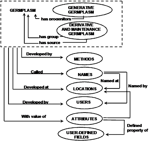
Pedigree information is stored independently of nomenclature making it uniform and amenable to computer manipulation. Strains are uniquely identified by germplasm identifiers (GID) and relate to source strains or progenitors depending on method of production. Methods are divided into three classes, maintenance methods (such as regeneration) designed to maintain genetic composition of a strain, generative methods (such as crossing) designed to increase genetic diversity and derivative methods (such as selection) designed to reduce and refine genetic diversity. The data model for genealogy information in ICIS is shown in Figure 1.
Strains produced by generative methods are linked to one or more progenitor strains: one progenitor in the case of mutants, two for bi-parental crossing schemes and more for dispersed mating schemes such as reciprocal recurrent selection. Strains produced by maintenance or derivative methods are linked to exactly one source strain and one group strain. The source strain is the immediately preceding generation and the group strain is the most recent generative generation in the pedigree of a strain. The source, or source and group may be unknown.
Information on nomenclature, origin and chronology are linked to the GID. Also users can define any attributes to be recorded and linked to GID. For example breeding objectives or conditions or intellectual property status of a strain could be stiored.
Computation of COP values by BROWSE
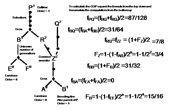
The BROWSE application of ICIS is a program which interacts with an ICIS database implementation for any crop to facilitate management and analysis of pedigree information. The computation of the COP between two strains in BROWSE commences with the extraction of the complete pedigree trees for two lines into a table with one row for each ancestor indicating: (1) its identity, (2) whether it is maintenance, derivative or generative germplasm, (3) the rows in the table for the source and group strains of the current ancestor if it is a derivative or maintenance strain or (4) the number of its progenitors, and (5) the row for the first progenitor if it is generative (further progenitors occur on subsequent rows of the table). As each ancestor is extracted, the table is checked to see whether that strain has already been tabulated as an ancestor of the first strain or from a different branch of the pedigree of the current strain. If so, pointers are set to the existing row and extraction of the branch is terminated.
The second step is to determine the order of the rows (ancestors) in the pedigree. This order is the largest number of generative steps from the current ancestor to a terminal ancestor via any of its progenitors. Terminal ancestors are those without progenitor information and in complete pedigrees should comprise landrace cultivars or wild relatives. Ancestors produced by derivative or maintenance methods have the same order as their group strains.
The third step is to use the recursive algorithm of equation 1 to accumulate COP values from terminal ancestors together with the relationships of equations 2 and 3 to incorporate inbreeding effects. An example is illustrated in Figure 2.
Contributions from Generative Processes
If P and Q are strains derived from different generative processes with known progenitors as in Figure 2, then Equation 1 is used. Although it is symmetrical in P and Q so that the parents of either could be used to obtain the right hand expansion, it is implemented in BROWSE by expanding the strain with the highest order. This ensures that when the terminal ancestors are reached, the computations involve COP values between the same strain, or unrelated strains or crosses between unrelated strains, all of which are easily calculated. If any parent is unknown, then COPs involving that parent are taken as zero.
Equation1 is generalized in BROWSE to allow generative processes involving any number of progenitors: If Q has progenitors Q1, Q2 … Qm then fPQ = (1/m) ∑ fPQi. This allows, for example, Q to be produced by a reciprocal recurrent selection program involving random mating between m strains. The current implementation assumes equal contribution from the m strains; but facilities exist in ICIS to record unequal contributions and the BROWSE computation could be easily generalized to obtain a differently weighted average.
Contributions from Inbreeding
If P and Q are derived from different generative strains, such as different crosses, the gametes of P and Q are essentially a random sample of the gametes from their group strains. Hence, the COP between P and Q is unaffected by inbreeding of P or Q and so it is ignored.
To compute the COP of a derivative strain with itself, say Z in Figure 2, the number of derivative generations from Z to its generative group, A ´ B, is counted and the inbreeding coefficient, FZ, of Z is determined by Equation 2 and converted to a COP using Equation 3.
BROWSE uses a parameter BTYPE to implement some assumptions in the case of incomplete pedigree records. The user should set BTYPE = 1 for self-pollinating species and 0 otherwise. If the progenitors of a strain are unknown, then FZ is set to BTYPE. This occurs most frequently when Z is derived from a landrace or traditional cultivar and corresponds to an assumption of full inbreeding for self-pollinating crops and no inbreeding for others. Similarly, if Z traces back to a single progenitor, such as a mutant strain, then FZ = BTYPE.
If there is a break in the records of source strains back to the group strain, as with strain B in Figure 2, then the strain is assumed to be an F4 derived breeding line so that FB = 1 – (1/2)4 = 15/16.
For strains which are sister lines derived from the same group, such as R and Q in Figure 2, the effect of inbreeding depends on the inbreeding coefficient of the most recent common ancestor, Z. If Z is the group strain of R and Q, then there is no effect of inbreeding. If incomplete pedigree records prevent the determination of a common ancestor, then R and Q are assumed to have diverged at the group strain. Otherwise, the gametes of R and Q can be regarded as a random sample of the possible gametes of Z and inbreeding since strain Z does not affect the COP. The inbreeding coefficient of Z and hence the COP between R and Q are computed as above with the same assumptions for strains with incomplete pedigrees.
COP matrices for all pairs of strains in a germplasm list
COP values are often required for all pairs of strains in a germplasm list. The matrix of these values indexed by strain is obviously symmetric with COPs for all strains with themselves on the diagonal. BROWSE implements this use-case by using the list processing facilities of ICIS. It extracts ancestors for all strains in the list into a single table as with pairs of strains. The program has a limit of 20,000 distinct ancestors for a single germplasm list. Since breeding populations are often highly related, this is not usually a constraint. The relatedness also implies that the same component ancestral COPs would be computed many times in calculating COPs for all pairs from the list. This is avoided by storing intermediate COP values for re-use in a sparse matrix with dimensions equal to the number of distinct ancestral strains. The COP algorithm checks this store whenever computations are required and writes to it whenever they have had to be executed.
Clearly, only one half of the COP matrix need be computed, and BROWSE outputs the lower triangular part, by rows as a list to the screen and to a text file. BROWSE also outputs this lower triangular matrix by rows in sections of ten columns at a time to the text file.
The inverse COP matrix is often required for mixed linear model analysis. BROWSE computes the eigen structure of the COP matrix pursuant to its inversion, and prints the eigen values and the first four eigen vectors of the COP matrix before inversion. The eigen vectors can be used to visualize and analyze the pedigree structure of the germplasm list.
Eigen values smaller than 1.0E-9 are taken to indicate singularities in the COP matrix (which occur, for example if the same strain occurs more than once in the list). The inverse COP matrix is computed from the eigen structure according to the formula:
![]() [5]
[5]
where li are the eigen values and ui the eigen vectors of A.
If A is singular, a G-Inverse A- is computed by omitting terms in the sum for which li < 1.0E-9.
The lower triangular part of the inverse (or G-inverse) is printed to the text output file by rows in sections of ten columns, and as a list by rows. The list contains row number, column number, matrix value, row-GID, column-GID for each cell of the lower triangular part of the matrix. This can readily be extracted and used in statistical software such as ASREML (Gilmour et al., 2006).
Visualization of COP matrices
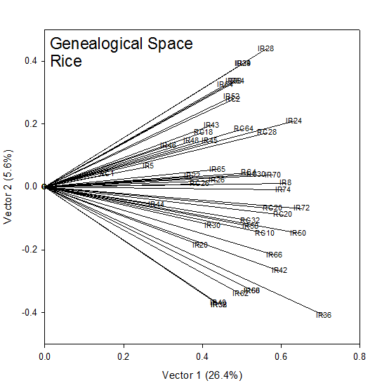
The eigen structure of the of the COP matrix used to obtain the inverse in Equation 5 can be used to construct ordination plots showing approximations to the additive genetic relationship between strains. The plotted points (√λ1ui1, √λ2ui2) in two dimensions or (√λ1ui1, √λ2ui2, √λ3ui3) in three dimensions display the rank 2 or rank 3 approximation to the COP matrix. The quality of the approximation can be gauged from the proportion of the generalized variance (sum of all the eigen values) accounted for by the first two or three eigen values. The approximation to fij shown in the plots is the inner product between the plotted vectors: ^f ij= (λ1ui1uj1+ λ2ui2uj2) or ^f ij= (λ1ui1uj1+ λ2ui2uj2+ λ3ui3uj3) and this is just √(^f ii ^f jj) Cos(θij) where θij is the angle subtended by the points for strains i and j at the origin. Hence if the diagonal elements of the COP matrix are constant, as in the case where the strains are all inbred lines then Cos(θij) is approximately proportional to the additive genetic correlation between strains i and j.
The COP matrix is a proximity matrix – the larger the values the closer the entities. Gower’s formula, dij = fij/√(fiifjj), can be used to transform it into a dissimilarity matrix and then cluster analysis by such methods as Ward’s agglomerative hierarchical clustering can be used to determine groups of closely related strains. The joint interpretation of the ordination plots and the cluster analysis is pattern analysis and is a powerful tool for summarizing high dimensional distance relationships.
The set of COP values between a strain which is a breeding line or cultivar and its terminal or founder strains which are often landrace cultivars of unknown parentage is called a Mendelgram. They give the proportion of alleles at unselected loci in the lines which are IBD from the founder and hence can be used to show the contribution of early germplasm to modern cultivars. These COP values for n lines with m distinct founders can be arranged in a Mendelgram Matrix, M, which contains information on the patterns of contribution of founders to lines. It can be subjected to Pattern Analysis to summariza and visualize these relationships. The n x m matrix M is factored by Singular Value Decomposition into three components, UΛV, where the columns of the n x p matrix U contain the left eigen vectors of M, and the rows of the p x m matrix V contain the right eigen vectors of M and the p x p diagonal matrix Λ contains the p non zero singular values of M, λk for k =1, 2, … p (p <= min(m,n)) in decreasing order of magnitude. The first two eigne vectors of each mode, lines and founders, are used to form a biplot. For the lines, spokes are plotted from the origin to the points (√λ1ui1, √λ2ui2), i=1, 2 .. n and the points (√λ1v1j, √λ2v2j) j=1, 2 … m. To the extent that the rank-two approximation ^mij= (λ1ui1v1j+ λ2ui2v2j) is close to M (as measured by the proportion of the generalized variance accounted for by the first two singular values), this is a picture of the Mendelgram Matrix. The projection of the founder point j onto the line spoke i is: ^mij/√( λ1ui12 + λ2ui22) so that the order of projections onto the spoke for any line gives the order of magnitudes of the contributions for the founters to that line. The greater the angle between the spokes for two lines, the more different will be this pattern of contributions.
The Euclidean distance between all pairs of lines (or founders) can be computed from the inner product of the rows (or columns) of the Mendelgram Matrix. These distance matrices can be subjected to cluster analysis to identify groups of lines receiving similar contributions from founders and groups of founders contributing similar proportions of alleles to lines. These groups can be interpreted with the biplot to give a Pattern Analysis of the Mendelgram Matrix.
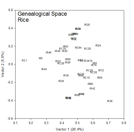
COP Analysis for the rice cultivars
The coordinates (√λ1u1i, √λ2u2i) for each cultivar, i, in Table 1 are plotted in Fig 1. The rank-two approximation to the COP matrix accounts for 32% of the generalized variance (sum of the eigen values). To the extent that this is a good approximation, this is a picture of the additive genetic relationships between the cultivars. IR28, IR29 and IR34 at the top of Figure 1 are highly related being sister lines from the same cross IR 2061. IR8 sits squarely in the center of the group and the vertical axis (Vector 2) measures genetic distance from IR8.
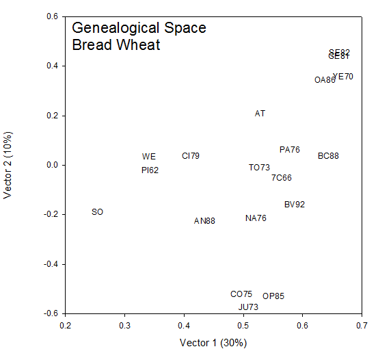
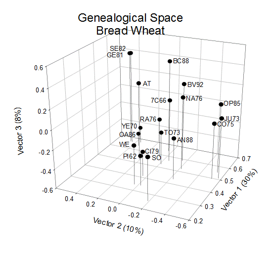
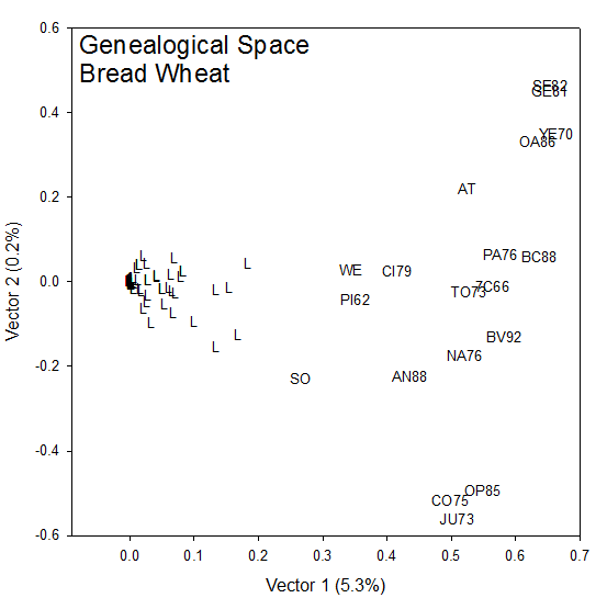
COP analysis of the wheat cultivars
Figure 2 shows a similar plot for the 19 wheat cultivars released in Mexico. In this case, however, the first three axes have been plotted to capture 48% of the generalized variance.
DISCUSSION
The BROWSE application and the ICIS database system make the routine computation of COP matrices possible for crop improvement programs.
The COP matrices or their inverses can be used for structural analysis of breeding nurseries, cross prediction strategies and for increasing the precision of estimates of breeding values. With database tools like ICIS and BROWSE linked to statistical software which is now available, this can be a routine part of any breeding program.
The ICIS software, including BROWSE, is freely available and published for use or further development through ICIS projects on CropForge at www.cropforge.org under the GNU open source license.
REFERENCES
Bernardo, R. 2002. Breeding for Quantitative Traits in Plants. Stemma Press. Woodbury, Minnesota, USA.
Burgueño, J., J. Crossa, P.L. Cornelius, R. Trethowan, G. McLaren and A. Krishnamachari. Modeling Additive ´ Environment and Additive ´ Additive ´ Environment Using Genetic Covariances of Relatives of wheat Genotypes. Crop Sci. (In Press).
Cowen, N.M. and K.J. Frey. 1978. Relationship Between Genealogical Distance and Breeding Behaviour in Oats (Avena Sativa L.). Euphytica 36:413-424.
Cox, T.S., Y.T. Kiang, M.B. Gorman, and D.M. Rodgers. 1985. Relationship Between Coefficient of Parentage and Genetic Similarity Indices in the soybean. Crop Sci. 25:529-532.
Crossa, R, J. Burgueño, P.L. Cornelius, G. McLaren, R. Trethowan, and A. Krishnamachari. 2006. Modeling Genotype ´ Environment Interaction Using Additive Genetic Covariance of Relatives for Predicting Breeding Values of Wheat Genotypes. Crop Sci. 46:1722-1733.
Dilday, R.H. 1990. Contribution of Ancestral Lines in the Development of New Cultivars of Rice. Crop Sci. 30:905-911.
Falconer, D.S. 1981. Introduction to Quantitative Genetics. Longman Group Ltd. Second Edition.
Fox, P.N. and B. Skovmand. The International Crop Information System (ICIS) – Connects Genebank to Breeder to Farmer’s Field. CAB International 1996. Plant Adaptation and Crop Improvement (eds. M. Cooper and G.L. Hammer).
Gilmour, A.R., Gogel, B.J., Cullis, B.R. and Thompson, R. 2006. ASReml User Guide Release 2.0. Department of Primary Industries, NSW, Australia
Hanson, W.D. 1994. Distance Statistics and Interpretation of Southern States Regional Soybean Tests. Crop Sci. 34:1498-1504.
Henderson, C.R. A simple methof for computing the inverse of a numerator relationship matrix used in predicting of breeding values. Biometrics 32: 69-83.
Lefort-Buson, M., Y. Dattee, and B. Guillot-Lemoine. 1986. Heterosis and Genetic Distance in Rapeseed (Brassica napus L.): use of Kinship Coefficient. Genome 29:11-18.
Lynch, M. And Walsh, B. 1998. Genetics and analysis of quantitative traits. Sinauer Associates, Massachusetts, U.S.A.
McLaren, C.G., R. Bruskiewich, A.M. Portugal, and A. B. Cosico. 2005. The International Rice Information system. A Platform for Meta-Analysis of Rice Crop Data. Plant Physiology 139:637-642.
Mrode, R.A. Linear Models for the Prediction of Animal Breeding Values. CAB International 1996.
Murphy, J.P., T.S. Cox, and D.M. Rodgers. 1986. Cluster Analysis of Red Winter Wheat Cultivars Based Upon Coefficients of Parentage. Crop Sci. 26:672-.
Sneller, C.H. 1994. Pedigree Analysis of Elite Soybean Lines. Crop Sci. 34:1515-1522.
Sneller, C.H. 1994. SAS Program for Calculating Coefficient of Parentage. Crop Sci. 34:1679-1680.
Souza, E., P.N. Fox, D. Byerlee, and B. Skovmand. 1994. Spring Wheat Diversity in Irrigated Areas of Two Developing Countries. Crop Sci. 34:774-783.
Tinker, N.A. and Mather, D.E. 1993. KIN:Software for computing kinship coefficients. J. Hered. 84:238.
Wright, S. 1922. Coefficients of inbreeding and relationship. Am.
Naturalist 56:330-338
CLUSTER |
ENTRYCD |
SOURCE |
DESIGNATION |
|
4 |
IR 29 |
IRRI |
IR 2061-464-4-14-1 |
|
4 |
IR 34 |
IRRI |
IR 2061-213-2-17 |
|
4 |
IR 28 |
IRRI |
IR 2061-214-3-8-2 |
|
4 |
RC 28 |
IRRI |
IR 56381-139-2-2, PSB RC 28, AGNO |
|
4 |
IR 64 |
IRRI |
IR 18348-36-3-3 |
|
4 |
IR 54 |
IRRI |
IR 5853-162-1-2-3 |
|
4 |
IR 52 |
IRRI |
IR 5853-118-5 |
|
4 |
IR 68 |
IRRI |
IR 28224-3-2-3-2 |
|
4 |
IR 65 |
IRRI |
IR 21015-196-3-1-3 |
|
|
|
|
|
|
1 |
IR 22 |
IRRI |
IR 579-160-2 |
|
1 |
IR 08 |
IRRI |
IR 8-288-3 |
|
1 |
IR 05 |
IRRI |
IR 5-47-2 |
|
1 |
IR 46 |
IRRI |
IR 2058-78-1-3-2 |
|
1 |
RC 01 |
IRRI |
IR 10147-113-5-1-1-5, PSB RC 1,MAKILING |
|
1 |
RC 18 |
IRRI |
IR 51672-62-2-1-1-2-3, PSB RC 18, ALA |
|
1 |
IR 48 |
IRRI |
IR 4570-83-3-3 |
|
1 |
IR 43 |
IRRI |
IR 1529-430-3 |
|
1 |
IR 24 |
IRRI |
IR 661-1-140-3-117,IR 661-1-140-3 |
|
1 |
IR 45 |
IRRI |
IR 2035-242-1 |
|
1 |
RC 26 H |
IRRI |
IR 64616 H, PSB RC 26 H, MAGAT |
|
1 |
IR 74 |
IRRI |
IR 32453-20-3-2-2 |
|
1 |
IR 70 |
IRRI |
IR 28228-12-3-1-1-2 |
|
1 |
IR 44 |
IRRI |
IR 2863-38-1-2 |
|
1 |
RC 64 |
IRRI |
IR 59552-21-3-2-2, PSB RC 64, KABACAN |
|
1 |
RC 02 |
IRRI |
IR 32809-26-3-3, PSB RC 2,NAHALIN |
|
|
|
|
|
|
3 |
RC 10 |
IRRI |
IR 50404-57-2-2-3, PSB RC 10, PAGSANJAN |
|
3 |
IR 66 |
IRRI |
IR 32307-107-3-2-2 |
|
3 |
RC 32 |
|
C 3563-B-5-1, PSB RC 32,JARO |
|
3 |
RC 52 |
IRRI |
IR 59682-132-1-1-2, PSB RC 52, GANDARA |
|
3 |
IR 50 |
IRRI |
IR 9224-117-2-3-3-2 |
|
3 |
RC 30 |
IRRI |
IR 58099-41-2-3, PSB RC 30, AGUS |
|
3 |
IR 72 |
IRRI |
IR 35366-90-3-2-1-2 |
|
3 |
RC 20 |
IRRI |
IR 57301-195-3-3, PSB RC 20, CHICO |
|
3 |
RC 04 |
IRRI |
IR 41985-111-3-2-2, PSB RC 4, MOLAWIN |
|
3 |
IR 42 |
IRRI |
IR 2071-586-5-6-3 |
|
3 |
IR 36 |
IRRI |
IR 2071-625-1-252 |
|
3 |
IR 58 |
IRRI |
IR 9752-71-3-2 |
|
3 |
IR 62 |
IRRI |
IR 13525-43-2-3-1-3-2 |
|
3 |
IR 60 |
IRRI |
IR 13429-299-2-1-3 |
|
3 |
IR 56 |
IRRI |
IR 13429-109-2-2-1 |
|
|
|
|
|
|
2 |
IR 30 |
IRRI |
IR 2153-159-1-4 |
|
2 |
IR 20 |
IRRI |
IR 532-E576,IR 532 E 576 |
|
2 |
IR 26 |
IRRI |
IR 1541-102-7 |
|
2 |
IR 38 |
IRRI |
IR 2070-423-2-5-6 |
|
2 |
IR 40 |
IRRI |
IR 2070-414-3-9 |
|
2 |
IR 32 |
IRRI |
IR 2070-747-6-3-2 |
Table 2. Wheat cultivars released in Mexico derived from CIMMYT breeding lines.
|
ENTRYID |
ENTRYCD |
SOURCE |
DESIGNATION |
|
1 |
PI62 |
MEXICO |
PITIC 62 |
|
2 |
7C66 |
MEXICO |
SIETE CERROS T 66 |
|
3 |
SO |
MEXICO |
SONALIKA |
|
4 |
YE70 |
MEXICO |
YECORA F 70 |
|
5 |
JU73 |
MEXICO |
JUPATECO F 73 |
|
6 |
TO73 |
MEXICO |
TORIM F 73 |
|
7 |
CO75 |
MEXICO |
COCORAQUE F 75 |
|
8 |
NA76 |
|
NACOZARI F 76 |
|
9 |
PA76 |
MEXICO |
PAVON F 76 |
|
10 |
CI79 |
MEXICO |
CIANO T 79 |
|
11 |
GE81 |
MEXICO |
GENARO T 81 |
|
12 |
SE82 |
MEXICO |
SERI M 82 |
|
13 |
OP85 |
MEXICO |
OPATA M 85 |
|
14 |
OA86 |
MEXICO |
OASIS F 86 |
|
15 |
AN88 |
MEXICO |
ANGOSTURA F 88 |
|
16 |
AT |
MEXICO |
ATTILA |
|
17 |
BC88 |
MEXICO |
BACANORA T 88 |
|
18 |
BV92 |
MEXICO |
BAVIACORA M 92 |
|
19 |
WE |
|
WEAVER |